Word2Vec explained - Assignment #5 - Udacity Deep Learning Course by Google

Hi,

I do have a good understanding of how vector spaces work (thanks to all the math I've learnt so far in undergrad and grad school). However, assignment #5 from Udacity's Deep Learning course was challenging to visualize and understanding the concept of how a group of vectors can successfully (or almost) represent words while reading them side-by-side as context. I watched a couple of videos and did a bunch of reading online before I attempted to solve the assignment.


Let me start by explaining the concept with an example. Consider this sentence:

Tommy the dog is my best friend.

As human - our understanding is that the sentence is referenced to a dog named tommy who is the writer/author's best friend.

How do you make a machine understand this by math?

Answer: Embeddings

Imagine each word of the above sentence as a cloud you use for association -  the visualization that comes to my mind is:

<Tommy><dog><best friend>  -- where < > represents one cloud.

Word2Vec is a technique which allows the machine to achieve this, the difference here is the position of each cloud in the space if a vector of dimension D. The goal is the take the input text, process it and make sure the deep learning algorithm organizes these words close to each other - associates them with a relation with each other. Their vectors in space are in close proximity of each other. This concept is known as embeddings.

There are 2 primary techniques mentioned in the assignment to achieve context learning from text.

1. Skip-gram Model

The way this model teaches association to the machine learning algorithm is by making pairs. From our sentence above. We aim to make (input,output) pairs like:

(Tommy,the)

(Tommy,dog)

(Tommy,best)

(Tommy,friend)

Note: Since Word2Vec is a method of unsupervised learning, there is no right answer provided to the computer for training. The input is streams (sentences of text) that are pre-processed in the form of pairs and fed to the network.

More Detail on each of these models (Visualization credit goes to thushv.com)-

V – Vocabulary Size (Number of unique words in the corpora)

P – The Projection or the Embedding Layer
D – Dimensionality of the Embedding Space
b – Size of a single Batch (batch_size)

t - target word (say Tommy in our case)

Figure on the left explains a top level architecture of the model, given a word(t) at the output you are given a bunch of words which are in close proximity in the embedding space.
Basically, if my input is Tommy I want to find out which other words make associative pairs with my given word - best, friend, dog

More on the implementation architecture (right side) image -

We feed batch size (b) vector with input words -
Batch contains b rows of : Inputs and Targets/Outputs (also known as Context and Target pairs)

• [0] Tommy (context) -  dog (target)

• [1] Tommy - best

• [2] Tommy - friend

• ...

• [b-1] .......

By choice, we select D as the dimension of vectors in the space to generate the embeddings.

At the output, of the embedding layer, an embedding is generated for the entire batch, this is passed through a "sampled softmax", Computing softmax against one hot pairs for the network can be computationally expensive. Especially while training both the positive and negative samples. In practice what we do is "sample" a subset of negatives given by the network to generate softmax outputs for them. This gives out a batch_size X V vector at the output. Please refer to my code for details on the implementation - I have tried to explain concepts in line through comments.

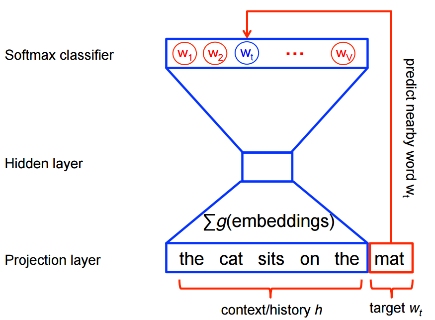
2. Continuous Bag of Words (CBoW)

Image source: Google Tensorflow

CBoW approach is like reverse(skip-gram) model. At the inputs, instead of providing the target words, we provide a group of context words and try to predict the target word. There is simply more information at the input here as compared to skip-gram (where you only have 1 word as the input). Hence, this model tends to do better.

Example of input to CBoW -
['dog','the','best','friend'] (Context) --- > ['Tommy'] (Target)

V – Vocabulary Size (Number of unique words in the corpora)

P – The Projection or the Embedding Layer
D – Dimensionality of the Embedding Space
b – Size of a single Batch (batch_size)

t - target word (say Tommy in our case)

As seen from the architecture the primary difference as compared to skip-gram model is that we compute separate embedding for each context word and average it out.

Input Layer comparison with Skip-Gram Model:

The input layer of skip-gram model was of dimension bx1:

(batch_size of words) - Each target word in a column

The input layer of CBoW is basically, batch_size x [context_window_size -1] (Not including the target word)

Source code with in-line comments:

Ankit AI Github

Resources - I do recommend watching these in order (I've arranged them in their order of complexity for ease of understanding)

• Udacity's short video on the concept: https://www.youtube.com/watch?v=xMwx2A_o5r4
• Andrew Ng's introduction to Word2Vec idea: https://www.youtube.com/watch?v=diUiV48q-5c
• Chris Manning (Stanford NLP) theory of Word2Vec: https://www.youtube.com/watch?v=ERibwqs9p38
• Diagram's are from Tushar's NLP Blog